Motion Detection with Path Tracking

Motion detection in a video footage has always been an interesting topic among the Machine Learning enthusiasts. It has many purposes. Motion detection can be used for automatic video analysis in video surveillance systems. It can be used to capture movements on a wildlife camera. Another application is to detect number of vehicles passing by on a highway.

In this article, we will build a fully working motion detector. It will not only detect motion, but will also be able to track motion of different objects. By this process, we will learn a lot about image processing techniques in OpenCV. By the end, you will have all the codes required to build your own motion detector.

Problem Statement

We will build a Computer Vision model for motion detection. It will be able to detect moving people in a video footage. Each person detected will have a different colored bounding box. The motion’s path will be shown with the same color as that of the bounding box.

We will achieve motion detection by comparing each video frame to the previous one. The spots which are different from the last frame are detected. For the predicting motion’s path, Kalman Filter is used. The final result will look like this:

Coding Our Motion Detector with Python

Firstly, we look at and understand the code for the motion detection. Then, we write scripts for tracking the path of moving objects. We will use the scripts and draw path of the objects on the frame. So, let’s begin-

1. Reading the video from location

We’ve used cv2.VideoCapture to capture the video from a file location. You can change it to your own location.

import cv2 
import imutils 
import numpy as np 
cap = cv2.VideoCapture('video.mp4')

2. Preparing the frames

while cap.isOpened():

# Capture frame-by-frame
    ret, frame = cap.read()
    if ret is None:
        break
    
    try:
        frame = imutils.resize(frame, width=750)
    except:
        break

    gray = cv2.cvtColor(frame, cv2.COLOR_BGR2GRAY)
    gray = cv2.GaussianBlur(gray, (21, 21), 0)

In this block of code, we capture each frame of the video and resize it. Then, we convert it to gray scale image. Now the frame’s pixels have values in the range of 0-255. Later, the frame is blurred to smooth it out a little.

3. Detecting motion in the frames

We begin with setting the first frame if it is None. If the number of frames exceed 5, we reset the delay counter and set the first frame with next frame.Motion is detected by comparing first frame with the next frame. The difference between frames is calculated using absdiff method.

if first_frame is None:
    first_frame = gray
next_frame = gray

delay_counter += 1

if delay_counter > 5:
    delay_counter = 0
    first_frame = next_frame

frame_delta = cv2.absdiff(first_frame, next_frame)
thresh = cv2.threshold(frame_delta, 25, 255, cv2.THRESH_BINARY)[1]

thresh = cv2.dilate(thresh, None, iterations=2)
cnts, _ = cv2.findContours(thresh.copy(), cv2.RETR_EXTERNAL, cv2.CHAIN_APPROX_SIMPLE)

threshold() method is used to make the pixels white whose values are greater than threshold value 25. The frames are dilated and we finally find the contours where motion is detected.

This is what it looks like-

5. Finding centroids of the objects in motion

For each contour with contour area greater than 1000, we find its centroid and store it. Simultaneously, we also store the coordinates of bounding box the centroid belongs to.

centers = []
coords = []
for c in cnts:
    try:
        (x, y, w, h) = cv2.boundingRect(c)
        if cv2.contourArea(c) > 1000:
            b = np.array([[x + w // 2], [y + h // 2]])
            centers.append(np.round(b))

            coords.append([x, y, x + w, y + h])
    except ZeroDivisionError:
        pass

We have successfully detected bounding boxes and their centroids for the motion detected in the video footage. So, the first half of our task is completed. Now, we proceed towards tracking the objects in motion.

Kalman Filter

Kalman filter algorithm estimates the states of a system given the observations or measurements. It is a useful tool for a variety of different applications including object tracking and autonomous navigation systems, economics prediction, etc.

The Kalman filter is essentially a set of mathematical equations that implement a predictor-corrector type estimator that is optimal in the sense that it minimizes the estimated error covariance when some presumed conditions are met [1].

Mathematical Equation [1]:

The Kalman filter addresses the general problem of trying to estimate the state x ∈ ℜn of a discrete-time controlled process that is governed by the linear stochastic difference equation

x= Axk-1 + Buk + wk-1

with a measurement m y ∈ℜ that is

y= Hxk +vk

The random variables wk and kv represent the process and measurement noise respectively. They are assumed to be independent of each other, white, and with normal probability distributions p(w) ≈ N ,0( Q) (3) p(v) ≈ N ,0( R)

The more detailed working of Kalman filter can be found in [1].

Tracking Path of Moving Object

We provide you with two python scripts named tracker.py and kalman_filter.py. The scripts contain codes to track the object with its centroid. It makes use of Kalman filter algorithm. The codes are explained within the scripts with the help of comments.

tracker.py

# Import python libraries
import numpy as np
from kalman_filter import KalmanFilter
from common import dprint
from scipy.optimize import linear_sum_assignment

class Track(object):
    """Track class for every object to be tracked
    Attributes:
        None
    """
    def __init__(self, prediction, trackIdCount):
        """Initialize variables used by Track class
        Args:
            prediction: predicted centroids of object to be tracked
            trackIdCount: identification of each track object
        Return:
            None
        """
        self.track_id = trackIdCount  # identification of each track object
        self.KF = KalmanFilter()  # KF instance to track this object
        self.prediction = np.asarray(prediction)  # predicted centroids (x,y)
        self.skipped_frames = 0  # number of frames skipped undetected
        self.trace = []  # trace path

class Tracker(object):
    """Tracker class that updates track vectors of object tracked
    Attributes:
        None
    """
    def __init__(self, dist_thresh, max_frames_to_skip, max_trace_length,
                 trackIdCount):
        """Initialize variable used by Tracker class
        Args:
            dist_thresh: distance threshold. When exceeds the threshold,
                         track will be deleted and new track is created
            max_frames_to_skip: maximum allowed frames to be skipped for
                                the track object undetected
            max_trace_lenght: trace path history length
            trackIdCount: identification of each track object
        Return:
            None
        """
        self.dist_thresh = dist_thresh
        self.max_frames_to_skip = max_frames_to_skip
        self.max_trace_length = max_trace_length
        self.tracks = []
        self.trackIdCount = trackIdCount

    def Update(self, detections):
        """Update tracks vector using following steps:
            - Create tracks if no tracks vector found
            - Calculate cost using sum of square distance
              between predicted vs detected centroids
            - Using Hungarian Algorithm assign the correct
              detected measurements to predicted tracks
              https://en.wikipedia.org/wiki/Hungarian_algorithm
            - Identify tracks with no assignment, if any
            - If tracks are not detected for long time, remove them
            - Now look for un_assigned detects
            - Start new tracks
            - Update KalmanFilter state, lastResults and tracks trace
        Args:
            detections: detected centroids of object to be tracked
        Return:
            None
        """
        # Create tracks if no tracks vector found
        if (len(self.tracks) == 0):
            for i in range(len(detections)):
                track = Track(detections[i], self.trackIdCount)
                self.trackIdCount += 1
                self.tracks.append(track)

        # Calculate cost using sum of square distance between
        # predicted vs detected centroids
        N = len(self.tracks)
        M = len(detections)
        cost = np.zeros(shape=(N, M))   # Cost matrix
        for i in range(len(self.tracks)):
            for j in range(len(detections)):
                try:
                    diff = self.tracks[i].prediction - detections[j]
                    distance = np.sqrt(diff[0][0]*diff[0][0] +
                                       diff[1][0]*diff[1][0])
                    cost[i][j] = distance
                except:
                    pass

        # Let's average the squared ERROR
        cost = (0.5) * cost
        # Using Hungarian Algorithm assign the correct detected measurements
        # to predicted tracks
        assignment = []
        for _ in range(N):
            assignment.append(-1)
        row_ind, col_ind = linear_sum_assignment(cost)
        for i in range(len(row_ind)):
            assignment[row_ind[i]] = col_ind[i]

        # Identify tracks with no assignment, if any
        un_assigned_tracks = []
        for i in range(len(assignment)):
            if (assignment[i] != -1):
                # check for cost distance threshold.
                # If cost is very high then un_assign (delete) the track
                if (cost[i][assignment[i]] > self.dist_thresh):
                    assignment[i] = -1
                    un_assigned_tracks.append(i)
                pass
            else:
                self.tracks[i].skipped_frames += 1

        # If tracks are not detected for long time, remove them
        del_tracks = []
        for i in range(len(self.tracks)):
            if (self.tracks[i].skipped_frames > self.max_frames_to_skip):
                del_tracks.append(i)
        if len(del_tracks) > 0:  # only when skipped frame exceeds max
            for id in del_tracks:
                if id < len(self.tracks):
                    del self.tracks[id]
                    del assignment[id]
                else:
                    dprint("ERROR: id is greater than length of tracks")

        # Now look for un_assigned detects
        un_assigned_detects = []
        for i in range(len(detections)):
                if i not in assignment:
                    un_assigned_detects.append(i)

        # Start new tracks
        if(len(un_assigned_detects) != 0):
            for i in range(len(un_assigned_detects)):
                track = Track(detections[un_assigned_detects[i]],
                              self.trackIdCount)
                self.trackIdCount += 1
                self.tracks.append(track)

        # Update KalmanFilter state, lastResults and tracks trace
        for i in range(len(assignment)):
            self.tracks[i].KF.predict()

            if(assignment[i] != -1):
                self.tracks[i].skipped_frames = 0
                self.tracks[i].prediction = self.tracks[i].KF.correct(
                                            detections[assignment[i]], 1)
            else:
                self.tracks[i].prediction = self.tracks[i].KF.correct(
                                            np.array([[0], [0]]), 0)
            if(len(self.tracks[i].trace) > self.max_trace_length):
                for j in range(len(self.tracks[i].trace) -
                               self.max_trace_length):
                    del self.tracks[i].trace[j]

            self.tracks[i].trace.append(self.tracks[i].prediction)
            self.tracks[i].KF.lastResult = self.tracks[i].prediction

kalman_filter.py

import numpy as np


class KalmanFilter(object):
    """Kalman Filter class keeps track of the estimated state of
    the system and the variance or uncertainty of the estimate.
    Predict and Correct methods implement the functionality
    Reference: https://en.wikipedia.org/wiki/Kalman_filter
    Attributes: None
    """
    def __init__(self):
        """Initialize variable used by Kalman Filter class
        Args:
            None
        Return:
            None
        """
        self.dt = 0.005  # delta time

        self.A = np.array([[1, 0], [0, 1]])  # matrix in observation equations
        self.u = np.zeros((2, 1))  # previous state vector

        # (x,y) tracking object center
        self.b = np.array([[0], [255]])  # vector of observations

        self.P = np.diag((3.0, 3.0))  # covariance matrix
        self.F = np.array([[1.0, self.dt], [0.0, 1.0]])  # state transition mat

        self.Q = np.eye(self.u.shape[0])  # process noise matrix
        self.R = np.eye(self.b.shape[0])  # observation noise matrix
        self.lastResult = np.array([[0], [255]])

    def predict(self):
        """Predict state vector u and variance of uncertainty P (covariance).
            where,
            u: previous state vector
            P: previous covariance matrix
            F: state transition matrix
            Q: process noise matrix
        Equations:
            u'_{k|k-1} = Fu'_{k-1|k-1}
            P_{k|k-1} = FP_{k-1|k-1} F.T + Q
            where,
                F.T is F transpose
        Args:
            None
        Return:
            vector of predicted state estimate
        """
        # Predicted state estimate
        self.u = np.round(np.dot(self.F, self.u))
        # Predicted estimate covariance
        self.P = np.dot(self.F, np.dot(self.P, self.F.T)) + self.Q
        self.lastResult = self.u  # same last predicted result
        return self.u

    def correct(self, b, flag):
        """Correct or update state vector u and variance of uncertainty P (covariance).
        where,
        u: predicted state vector u
        A: matrix in observation equations
        b: vector of observations
        P: predicted covariance matrix
        Q: process noise matrix
        R: observation noise matrix
        Equations:
            C = AP_{k|k-1} A.T + R
            K_{k} = P_{k|k-1} A.T(C.Inv)
            u'_{k|k} = u'_{k|k-1} + K_{k}(b_{k} - Au'_{k|k-1})
            P_{k|k} = P_{k|k-1} - K_{k}(CK.T)
            where,
                A.T is A transpose
                C.Inv is C inverse
        Args:
            b: vector of observations
            flag: if "true" prediction result will be updated else detection
        Return:
            predicted state vector u
        """

        if not flag:  # update using prediction
            self.b = self.lastResult
        else:  # update using detection
            self.b = b
        C = np.dot(self.A, np.dot(self.P, self.A.T)) + self.R
        K = np.dot(self.P, np.dot(self.A.T, np.linalg.inv(C)))

        self.u = np.round(self.u + np.dot(K, (self.b - np.dot(self.A,
                                                              self.u))))
        self.P = self.P - np.dot(K, np.dot(C, K.T))
        self.lastResult = self.u
        return self.u

Now, in the final part of the article, we will first draw tracking lines. Then, we draw bounding boxes for each object. The color of bounding box and tracking lines will be same and unique for each object.

We begin with importing Tracker class from the tracker.py script. We write the following code before the while loop i.e. before while cap.isOpened():-

from tracker import Tracker
traces = []
tracker = Tracker(200, 30, 20, 100)
# Variables initialization
skip_frame_count = 0
track_colors = [(255, 0, 0), (0, 255, 0), (0, 0, 255), (255, 255, 0),
                (0, 255, 255), (255, 0, 255), (255, 127, 255),
                (127, 0, 255), (127, 0, 127)]

After adding this code, we proceed to write code within the while loop i.e. within while cap.isOpened() loop.

# If centroids are detected then track them
if len(centers) > 0:

    # Track object using Kalman Filter
    tracker.Update(centers)

    # For identified object tracks draw tracking line
    # Use various colors to indicate different track_id
    colors = {}
    for i in range(len(tracker.tracks)):
        if len(tracker.tracks[i].trace) > 1:
            for j in range(len(tracker.tracks[i].trace) - 1):
                # Draw trace line
                x1 = tracker.tracks[i].trace[j][0][0]
                y1 = tracker.tracks[i].trace[j][1][0]
                x2 = tracker.tracks[i].trace[j + 1][0][0]
                y2 = tracker.tracks[i].trace[j + 1][1][0]
                clr = tracker.tracks[i].track_id % 9
                traces.append([x1,y1,x2,y2,clr])
            for trace in traces:
                frame = cv2.line(frame, (int(trace[0]), int(trace[1])), (int(trace[2]), int(trace[3])),
                         track_colors[trace[4]], 2)
            if clr not in colors.keys():
                colors[clr] = [x2, y2]

            try:
                c = []
                for z in range(len(coords)):
                    minv = np.linalg.norm(np.array(centers[z]) - np.array(list(colors.values())[0]))
                    v = list(colors.keys())[0]

                    for val in range(1, len(colors.keys())):
                        dist = np.linalg.norm(np.array(centers[z]) - np.array(list(colors.values())[val]))
                        if dist < minv:
                            minv = dist
                            v = list(colors.keys())[val]
                    if v in c:
                        c.append(v + 1)
                    else:
                        c.append(v)
                for z in range(len(coords)):
                    cv2.rectangle(frame, (coords[z][0], coords[z][1]), (coords[z][2], coords[z][3]),
                                  track_colors[c[z]], 2)

            except:
                pass

The above code block successfully draws tracking paths and bounding boxes on the frame. The frame can be shown using imshow() method.

Conclusion

In this article, we’ve examined how motion detection works in a video. We also worked with image processing techniques like blurring, diluting, finding differencesbetween frames. In addition, we saw how Kalman filter can be used to track the moving objects. At last, we learned about drawing bounding boxes and lines on the image with unique colors.

References

[1]. Mohamed LAARAIEDH. “Implementation of Kalman Filter with Python Language“. IETR Labs, University of Rennes 1. https://arxiv.org/ftp/arxiv/papers/1204/1204.0375.pdf

Implement Non-linear Independent Components Estimation with Tensorflow

Non-Linear Independent Components Estimation

Non-linear Independent Components Estimation is a normalizing flow-based generative model which is used to learn the probability distribution of the real samples and then generate the new sample data. This algorithm can be categorized as generative models as GAN and VAE but using a different approach conceptually. While GAN doesn’t impose a prior distribution and VAE approximates the prior distribution, This NICE algorithm estimates the real distribution to which real data belongs. This tutorial is a step-by-step guide to understand the non-linear independent components estimation algorithm and write the code using Tensorflow 2.0.

Introduction

In the normalizing flow method, The probability distribution p(x) is a composition of differentiable bijective functions f.p(x)=f0∗f1∗f2∗f3….fkp(x)=f0​∗f1​∗f2​∗f3​….fk

Here each function f should have following characteristics –

  • Easy to differentiable
  • Easy to compute the determinant of Jacobian of function f
  • And f should be invertible.

The objective of the NICE model is to learn these factorial functions f using a neural network and then use these model training parameters to generate new data. The loss criteria are maximum log-likelihood using the change of variable equation.logPX(x)=logPz(f(x))+log(∣det(∂(f(x))∂(x))∣)logPX​(x)=logPz​(f(x))+log(∣det(∂(x)∂(f(x))​)∣)

Here Pz(f(x))Pz​(f(x)) is a prior distribution and ∂(f(x))∂(x)∂(x)∂(f(x))​ is Jacobian matrix of function f at x.

So we’re trying to represent the complex non-linear distribution as a simpler prior distribution.

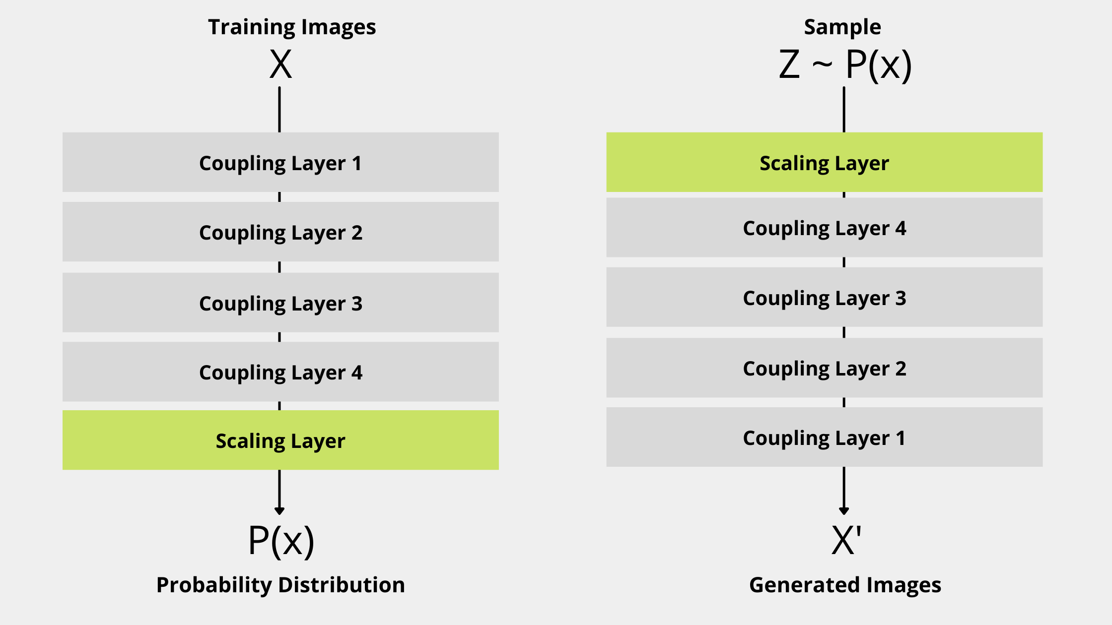
The NICE model has Coupling Layer and Scaling Layer as the main components in its architecture.

Coupling Layer

The NICE model has multiple coupling layer and each coupling layer represent a function f. So f0,f1,f2,f3….fkf0​,f1​,f2​,f3​….fk​ are coupling layers. if X is input to a coupling layer then output Y is defined where:y1=x1y1=x1y2=g(x2;m(x1))y2=g(x2;m(x1))

Here x1 and x2 are partitions of the input X and function m is a non-linear neural network.

The Jacobian of f at x is defined as below:[∂y1∂x1∂y1∂x2∂y2∂x1∂y2∂x2][∂x1∂y1​∂x1∂y2​​∂x2∂y1​∂x2∂y2​​]

In this tutorial, we use additive coupling layer as g function.y1=x1y1=x1y2=x2+m(x1)y2=x2+m(x1)

Note that y2 depends on both x1 and x2 but y1 only depends on x1. so The Jacobian will be:[10∂y2∂x11][1∂x1∂y2​​01​]

This is a lower triangle matrix hence its determinate will be the product of the diagonal elements. so Jacobian of additive coupling layer will be 1 always hence it’s a volume-preserving operation.

Each coupling layer unchanged some part of the input so we combine multiple coupling layers so all inputs elements can be modified.

Scaling Layer

The additive coupling layer is a volume-preserving operation so the composition of all coupling layers will also be a volume-preserving operation which is a problem in a real-life data transformation. Without changing volume of a unknown complex distribution, we can’t transform it to a much simpler distribution. So we introduce a new layer as the output layer of the NICE model architecture which allows us to give more weights to some dimensions and less to others hence more weight variations. So we add a diagonal layer S which transforms the output of coupling layers.(xi)i<=D→(Siixi)i<=D(xi​)i<=D​→(Siixi​)i<=D

NICE Model Architecture

This is the last part we need to discuss before start writing the code. In this tutorial, we’ll use MNIST database as training input and will have following architectural decisions.

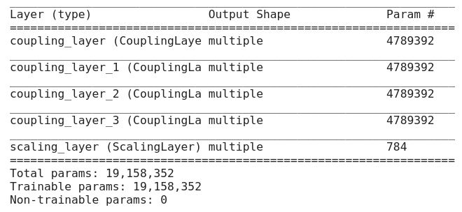
  • It has 4 Coupling Layers. Each coupling layer consists of Sequential Model which has 1000 units in hidden layers.
  • It has 1 scaling layer consists of [1,784] random values from a uniform distribution.
  • Maximum loglikelihood as loss function.
  • Adam optimizer to update the parameters in backpropagation.

TensorFlow 2.0 Code

Below is the step-by-step guide to implementing the Non-Linear Independent Components Estimation algorithm with TensorFlow. Each line is well commented.

First thing first, load the require libraries.

import tensorflow as tf
from tensorflow import keras
from tensorflow.keras import layers
from tensorflow.keras.datasets import mnist
import numpy as np
import matplotlib.pyplot as plt

Define Coupling Layer

class CouplingLayer(layers.Layer):

	""" This method define the neural network to learn function F

    Parameters
    ----------
    input_dim : int
        - Number of Pixels - width * height
    hidden_dim : int
        - Number of Units per hidden layer
    partition : String
        - Odd or even indexing scheme
    num_layers : int
        - Number of hidden layer
    
    """

	def __init__(self,input_dim, hidden_dim, partition, num_hidden_layers):
		
		super(CouplingLayer, self).__init__()

		assert input_dim % 2 == 0

		self.partition = partition # Posssible values - odd or even

		# Define Neural Network

		inputs = keras.Input(shape = (input_dim))
		
		x = inputs
		for layer in range(num_hidden_layers):
			x = layers.Dense(hidden_dim)(x)
			x = layers.LeakyReLU()(x)

		outputs = layers.Dense(input_dim, activation='linear')(x)
		self.m = keras.Model( inputs = inputs, outputs = outputs)

		# Define lambda functions to get odd or even indexed data.
		if self.partition == 'even':
			self._first = lambda xs: xs[:,0::2]
			self._second = lambda xs: xs[:,1::2]
		else:
			self._first = lambda xs: xs[:,1::2]
			self._second = lambda xs: xs[:,0::2]

	""" This method implement additive coupling layer operations. 
	y1 = x1
	y2 = x2 + m(x1)

    Parameters
    ----------
    inputs : Tensor Array
        Input Tensors.

    Returns
        -------
        Tensor Array
            Latent representation.
    """

	def call(self,inputs):

		# Split input into two parts x1 and x2
		x1 = self._first(inputs)
		x2 = self._second(inputs)
		
		# Inference latent representation
		y1 = x1
		y2 = x2 + self.m(x1)
		
		# Merge both y1 an y2 using interleave method. e.g y1 = [1,3,5,7,9] and y2 = [2,4,6,8,10] then y = [1,2,3,4,5,6,7,8,9,10]
		if self.partition == 'even':
		      y = tf.reshape(tf.concat([y1[...,tf.newaxis], y2[...,tf.newaxis]], axis=-1), [tf.shape(y1)[0],-1])
		else:
		      y = tf.reshape(tf.concat([y2[...,tf.newaxis], y1[...,tf.newaxis]], axis=-1), [tf.shape(y2)[0],-1])
		return y

	"""This function will generate new image using latent variable

    Parameters
    ----------
    latent_variable : Tensor Array
       . latent variable from logistic distribution.
    
    Returns
    -------
    List
        Pixels value.
    """
	def inverse(self,latent_variable):

		y1 = self._first(latent_variable)
		y2 = self._second(latent_variable)
		x1,x2 = y1, y2 - self.m(y1)

		if self.partition == 'even':
		      x = tf.reshape(tf.concat([x1[...,tf.newaxis], x2[...,tf.newaxis]], axis=-1), [tf.shape(x1)[0],-1])
		else:
		      x = tf.reshape(tf.concat([x2[...,tf.newaxis], x1[...,tf.newaxis]], axis=-1), [tf.shape(x2)[0],-1])

		return x

Define Scaling Layer

class ScalingLayer(layers.Layer):
	""" This method define the scaling layer with normal distribution.

	Parameters
	----------
	input_dim : int
	- Number of Pixels - width * height
	"""
	def __init__(self,input_dim):
		super(ScalingLayer,self).__init__()
		self.scaling_layer = tf.Variable(tf.random.normal([input_dim]),trainable=True)

	""" This method rescale the final out of coupling layers.

	Parameters
	----------
	x : Tensor Array
	- Tensors to be rescale.
	"""
	def call(self,x):
		return x*tf.transpose(tf.math.exp(self.scaling_layer))

	""" This method is inverse implementation of the call method.

	Parameters
	----------
	z : Tensor Array
	    - Tensors to be rescale.
	"""
	def inverse(self,z):
	    return z*tf.transpose(tf.math.exp(-self.scaling_layer))

Define NICE Model

class NICE(keras.Model):

	""" This function define trainable model with multiple coupling layers and a scaling layer.

    Parameters
    ----------
    input_dim : int
        - Number of Pixels - width * height
    hidden_dim : int
        - Number of Units per hidden layer
    num_hidden_layers : int
        - Number of hidden layer
    
    """

	def __init__(self,input_dim,hidden_dim,num_hidden_layers):

		super(NICE,self).__init__()
		self.input_dim = input_dim
		# Coupling layer will have half dimension of the input data.
		half_dim = int(self.input_dim / 2)

		# Define 4 coupling layers.
		self.coupling_layer1 = CouplingLayer(input_dim=half_dim, hidden_dim = hidden_dim, partition='odd', num_hidden_layers=num_hidden_layers)
		self.coupling_layer2 = CouplingLayer(input_dim=half_dim, hidden_dim = hidden_dim, partition='even', num_hidden_layers=num_hidden_layers)
		self.coupling_layer3 = CouplingLayer(input_dim=half_dim, hidden_dim = hidden_dim, partition='odd', num_hidden_layers=num_hidden_layers)
		self.coupling_layer4 = CouplingLayer(input_dim=half_dim, hidden_dim = hidden_dim, partition='even', num_hidden_layers=num_hidden_layers)
		
		# Define scaling layer which rescaling the output for more weight variations.
		self.scaling_layer = ScalingLayer(self.input_dim)

	"""This function calculates the log likelihood.

    Parameters
    ----------
    z : Tensor Array
        Latent space representation.

    Returns
        -------
        List
            Log likelihood.
    """

	def log_likelihood(self, z):
		log_likelihood = tf.reduce_sum(-(tf.math.softplus(z) + tf.math.softplus(-z)), axis=1) + tf.reduce_sum(self.scaling_layer.scaling_layer)
		return log_likelihood

	""" This function passes input through coupling layer. Scale the output using scaling layer and return latent space z and loglikelihood

    Parameters
    ----------
    x : Tensor Array
        Input data from training samples.

    Returns
        -------
        Tensor Array
            Latent space representation.
        List
        	Log-likelihood for each image in the batch
    """

	def call(self, x):
		
		z = self.coupling_layer1(x)
		z = self.coupling_layer2(z)
		z = self.coupling_layer3(z)
		z = self.coupling_layer4(z)
		z = self.scaling_layer(z)

		log_likelihood = self.log_likelihood(z)
		return z,log_likelihood

	""" Generate sample data using latent space. This is exact inverse of the call method.

    Parameters
    ----------
    z : Tensor Array
        Latent Spaec.

    Returns
    -------
    Tensor Array
        Newly generated data
    """

	def inverse(self,z):
		x  = z
		x  = self.scaling_layer.inverse(x)
		x  = self.coupling_layer4.inverse(x)
		x  = self.coupling_layer3.inverse(x)
		x  = self.coupling_layer2.inverse(x)
		x  = self.coupling_layer1.inverse(x)

		return x

	""" Sample out new data from learnt probability distribution

    Parameters
    ----------
    num_samples : int
        - Number of sample images to generate.

    Returns
    -------
    List
    	- List of generated sample data.
        
    """

	def sample(self, num_samples):
		z = tf.random.uniform([num_samples, self.input_dim])
		z = tf.math.log(z) - tf.math.log(1.-z)
		return self.inverse(z)

Train NICE Model

Basic model configurations.

input_data_size = 784 # for mnist dataset. 28*28
num_epochs = 100
batch_size = 256
num_hidden_layer = 5
num_hidden_units = 1000

Prepare training dataset.

# Prepare training dataset
(x_train, y_train), (x_test, y_test) = mnist.load_data()
x_train = (x_train.reshape(-1,input_data_size) + tf.random.uniform([input_data_size])) / 256.0
dataloader = tf.data.Dataset.from_tensor_slices((x_train, y_train)).batch(batch_size)

Define a function show_samples() to generate sample images after certain epochs.

def show_samples():
    # Generate 100 sample digits
    ys = model.sample(21)
    plt.figure(figsize=(5, 5))
    plt.rcParams.update({
        "grid.color": "black",
        "figure.facecolor": "black",
        "figure.edgecolor": "black",
        "savefig.facecolor": "black",
        "savefig.edgecolor": "black"})
    new_images = tf.reshape(ys,(-1,28,28))
    for i in range(1,20):
      plt.subplot(2,10,i)
      plt.axis('off')
      plt.imshow(new_images[i],cmap="gray")
    plt.show()

Start custom training loop now.

model = NICE(input_dim = input_data_size, hidden_dim = num_hidden_units, num_hidden_layers = num_hidden_layer)

opt = keras.optimizers.Adam(learning_rate=0.001,clipnorm=1.0)

# Iterate through training epoch
for i in range(num_epochs):

	# Iterate through dataloader
	for batch_id,(x,_) in enumerate(dataloader):

		# Forward Pass
		with tf.GradientTape() as tape:
			z, likelihood = model(x)
			log_likelihood_loss = tf.reduce_mean(likelihood)
			# Convert the maximum likelihood problem into negative of minimum likelihood problem
			loss = -log_likelihood_loss
		# Backward Pass
		gradient = tape.gradient(loss,model.trainable_weights)
		opt.apply_gradients(zip(gradient,model.trainable_weights))

	# Log the maxmimum likelihood after each training loop
	print('Epoch {} completed. Log Likelihood:{}'.format(i,log_likelihood_loss))
	# Generate 20 new images after 10 epochs.
	if i % 10 == 0 and i!=0:
		show_samples()

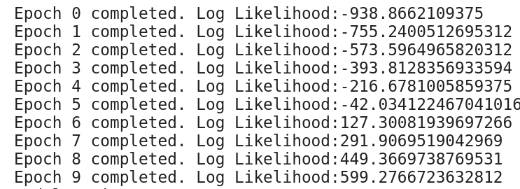
Here are the log of first 10 epochs.

Please read the original paper for a depth understanding. and here is the Github repo Non-Linear Independent Components Estimation with Tensorflow to start playing with the code.